
ResonantGSER Layer
The recurrent feedback layer at the core of ARCANE's adaptive System 1 architecture.
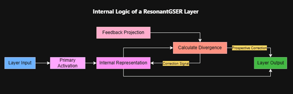
Figure 1: Internal logic and state synchronization of the ResonantGSER layer.
Overview
ResonantGSER (Resonant Gated Spiking Elastic Reservoir) is the recurrent feedback layer at the core of ARCANE's adaptive System 1 architecture. Its current-input path uses explicit per-example top-down targets while keeping learned weights fixed. Separate APIs train feedback projections or perform bounded objective-driven test-time weight adaptation.
Biological Inspiration
ResonantGSER draws inspiration from several key biological neural processes:
Predictive Coding
The brain constantly generates predictions about sensory inputs and compares them with actual inputs, minimizing prediction errors through hierarchical feedback loops.
Hierarchical Processing
Cortical processing occurs across multiple hierarchical levels, with higher areas providing contextual expectations that modulate lower-level processing.
Adaptive Resonance Theory (ART)
Adaptive Resonance Theory motivates the stability/plasticity framing. Evaluate retention alongside task quality when using ResonantGSER in continual-learning workflows.
Bi-directional Cortical Communication
The neocortex features extensive feedback connections that are as numerous as feedforward connections, enabling top-down contextual influence.
Core Concept
ResonantGSER supports an explicit refinement phase before final predictions are returned. Instead of a single evaluation, the wrapper can run multiple cycles on the same current input:
- Feedforward Pass: Initial processing through hierarchical layers
- Resonance Cycles: Iterative feedback and harmonization
- State Alignment: Layers synchronize representations
- Cycle Selection: Return predictions from the lowest-divergence observed cycle
Mathematical Formulation
Harmonization is one EMA step toward the top-down projection :
cycles have the closed form
The cell evaluates this closed form rather than an unrolled Python loop. If no alignment has been set (zero vector and alignment_set == 0), the resonance step is skipped so the first forward pass is not attracted to the origin.
project_feedback(state) maps within hidden space (projection_kernel). project_feedback(state, to_input_space=True) uses feedback_weights to reconstruct the cell's input dim.
Scope: predict_with_resonance extracts one state per example and carries ephemeral targets of shape (batch, units) through each refinement call. resonance_alignment and last_h remain batch-mean compatibility summaries for legacy manual/callback APIs; the explicit inference loop does not read those summaries.
Resonance Cycle (callback / run_resonance_cycle)
At each outer cycle the orchestrator performs:
predict_with_resonance performs a forward initialization and re-runs the current input after every harmonization step. NeuralResonanceCallback, by contrast, runs on on_train_batch_begin, so it can only stage the previous batch prototype; it is not a full current-batch RSAA inner loop.
Where:
- : Semantic representation at layer
- : Top-down projection from layer to
- : Prediction divergence (error signal)
- : Resonance factor
- : Semantic divergence weight
- : Clipped step size
Spiking Mechanism
ResonantGSER fires graded spikes against a self-scaling threshold. is relative: each state fires against , emits a signed spike count, and transmits count :
Each unit learns its own (initialised at spike_threshold) and a leak that passes of the sub-quantum remainder through. Negative counts are inhibitory spikes and large values burst. The backward pass is the identity with respect to , so there is no dead band at the threshold, and a learnable still receives a gradient.
Implementation in ARCANE
ResonantGSERCell
The fundamental building block implementing resonance dynamics:
cell = ResonantGSERCell( units=128, # Hidden units resonance_factor=0.2, # Resonance strength (γ) spike_threshold=0.5, # Spiking threshold (θ) resonance_cycles=5, # Maximum resonance iterations convergence_epsilon=1e-4, # Convergence criterion (ε) semantic_divergence_weight=0.1 # Semantic weighting (β))Key Components:
- LSTM Base: Standard LSTM for temporal processing
- Resonance Gate: Learned modulation of resonance strength
- Projection kernel: Hidden-space top-down map used by
project_feedback() - Feedback weights: Input-space reconstruction via
project_feedback(..., to_input_space=True) - State Tracking: the probe exposes per-example sequence means;
last_his only their compatibility summary
ResonantGSER Layer
RNN wrapper providing hierarchical integration:
layer = ResonantGSER( units=128, resonance_factor=0.2, resonance_cycles=5, return_sequences=False, # Single output or sequence return_state=False # Include final states)Hierarchical Features:
- Layer Linking:
set_higher_layer()andset_lower_layer() - Feedback Projection:
project_feedback()for top-down signals - State Harmonization:
harmonize_states()for bottom-up alignment
PredictiveResonantLayer: Local Predictive Resonance
For sequence models that do not require cross-layer hierarchical wiring, ARCANE provides PredictiveResonantLayer, which implements local predictive resonance in a self-contained RNN:
- Per-example alignment: Alignment is part of the recurrent state
(h, c, align), not a single global vector. Each sequence has its own resonance target. - No external callbacks: The layer does not depend on model references or custom training callbacks; it resonates toward an internal slow-moving prediction of future activity.
- Optional stateful resonance: Set
persist_alignment=Trueso alignment state carries across separate forward passes (e.g. repeated inference on the same or different inputs), enabling inference-time state adaptation. - Typical use: Sequence classification (e.g. MNIST as 28 time steps), when you want predictive-coding-style resonance without configuring a hierarchy of ResonantGSER layers.
from gpbacay_arcane import PredictiveResonantLayerlayer = PredictiveResonantLayer( units=128, resonance_cycles=3, resonance_step_size=0.2, spike_threshold=0.4, return_sequences=True, persist_alignment=False # True for stateful resonance across calls)Combine with BioplasticDenseLayer(..., enable_inference_plasticity=True) for inference-time Hebbian plasticity in the same model.
Integration in Models
NeuromimeticSemanticModel
ResonantGSER layers are integrated throughout the semantic foundation model:
# Multi-layer hierarchical resonancegser1 = ResonantGSER(units=256, resonance_factor=0.15, resonance_cycles=3)gser2 = ResonantGSER(units=128, resonance_factor=0.2, resonance_cycles=5)gser3 = ResonantGSER(units=64, resonance_factor=0.25, resonance_cycles=7)# Establish hierarchical relationshipsgser1.set_higher_layer(gser2)gser2.set_lower_layer(gser1)gser2.set_higher_layer(gser3)gser3.set_lower_layer(gser2)# Model architecturex = gser1(inputs)x = gser2(x)outputs = gser3(x)Neural Resonance Training
Integration with the NeuralResonanceCallback for training:
# During training, resonance cycles are orchestratedcallback = NeuralResonanceCallback( resonance_cycles=5, learning_rate=0.01, resonant_layers=[gser1, gser2, gser3])model.fit(x_train, y_train, callbacks=[callback])Validation and Testing
Unit tests in tests/test_resonant_gser.py and tests/test_mechanism_correctness.py cover:
ResonantGSER Cell Basic Functionality: state managementResonance Convergence: divergence decreases over harmonization stepsHierarchical Resonance: set_higher_layer / set_lower_layer after build (Keras 3)Divergence Computation: Δ = S - PLayer Integration: compiles inside a Keras ModelZero-alignment skip: first forward pass is not pulled toward the originRun:
python -m pytest tests/test_resonant_gser.py tests/test_mechanism_correctness.py -qconvergence_epsilon is stored on the cell and used by HierarchicalResonanceFoundationModel.run_resonance_cycle() for outer early-stop. The inner cell step is closed-form and does not early-break.
Parameter Sensitivity
| Parameter | Practical Range | Effect |
|---|---|---|
resonance_factor | 0.15 - 0.30 | Larger α moves faster toward ; clipped below 0.99 |
resonance_cycles | 3 - 8 | Appears in the closed-form exponent |
spike_threshold | 0.3 - 0.7 | Relative threshold (fraction of mean abs state); smaller = more spikes |
convergence_epsilon | 1e-6 - 1e-3 | Outer-loop stop in run_resonance_cycle |
Visual Analysis
Convergence Trajectories
The test suite generates detailed visualizations showing:
Resonance Cycle Convergence
- Divergence reduction over 15 iterations
- Exponential convergence to target alignment
- Parameter sensitivity across different configurations
Hierarchical State Alignment
- Multi-layer representation synchronization
- Feedback projection effectiveness
- Cross-layer coherence development
Parameter Optimization
- Convergence rate vs resonance factor relationships
- Error decay analysis with logarithmic scaling
- Statistical performance summaries
Benefits for Neural Networks
Overcoming Feedforward Limitations
- Iterative alignment: Hidden states can move toward a top-down prototype before the next forward pass
- Hierarchical wiring:
set_higher_layer/set_lower_layerconnect projection and harmonization - Local predictive variant:
PredictiveResonantLayerkeeps alignment per example in RNN state
The closed-form step is a state smoother, not a hidden reasoning loop. Treat it as bounded System 1 refinement and evaluate whether it improves the direct task output.
Implemented capabilities
- Per-example refinement: top-down targets retain the batch dimension
- Differentiable feedback training: explicit reconstruction/alignment loss updates projection kernels
- Bounded test-time adaptation: objective-driven updates support rollback and episodic reset
- Controlled evaluation: the ablation harness measures quality, calibration, latency, forgetting, order, batching, and shift
Usage Guidelines
Architecture Design
- Layer Hierarchy: Tune hierarchy depth as a task-specific configuration
- Parameter Tuning: Start with
resonance_factor=0.2, then evaluate downstream metrics - Cycle Count: Compare 0, 1, 2, 4, and 8 cycles from the same checkpoint
- Integration Points: Use in intermediate layers for semantic processing
Training Considerations
- Feedback Training: Use
train_feedback_stepwhen learned feedback projections should receive an explicit alignment gradient; retain the callback only for legacy previous-batch experiments - Learning Rate: Coordinate with overall model learning rate
- Batch Size: Per-example targets should be invariant to co-batching; measure this with the ablation harness because floating-point kernels can still introduce tiny numerical differences
- Sequence Length: Profile latency and memory at the lengths required by the task
Performance Optimization
- Closed-form inner step: The cell no longer unrolls Python iterations.
- Outer early stop:
run_resonance_cyclecan halt when summed divergenceconvergence_epsilon. - Do not pull to zero: Resonance is skipped until
harmonize_states(or a non-zero alignment) has run.
What this mechanism is not
ResonantGSER does not re-run the network on the current batch inside NeuralResonanceCallback; that legacy callback still stages a batch-mean prototype. predict_with_resonance is the per-example current-input path. Claims of general reasoning, multi-modal unification, or task gains are hypotheses, not results of the unit tests. The implemented claim is narrower: bounded recurrent refinement for a System 1 prediction.
Future work
- Evaluate whether lower reconstruction error predicts better downstream metrics.
- Compare learned, tied, and identity feedback projections.
- Make
GSER.prune_neuronsgraph-safe; it still uses a Python swap-remove.
References
Biological Foundations
- Predictive Coding: Rao, R. P., & Ballard, D. H. (1999). Nature Neuroscience
- Hierarchical Processing: Felleman, D. J., & Van Essen, D. C. (1991). Cerebral Cortex
- Adaptive Resonance: Grossberg, S. (2013). Frontiers in Psychology
Computational Implementations
- Hierarchical Resonance: RSAA notes in
docs/NEURAL_RESONANCE.md - Linear kernel attention: Katharopoulos et al., Transformers are RNNs (2020)
This documentation matches the ResonantGSER implementation in ARCANE after the 2026 mechanism corrections.