
Hierarchical Neural Resonance
Top-down feedback that aligns per-example state before a System 1 model commits to an output.
Overview
Hierarchical Neural Resonance aligns recurrent hidden states with per-example top-down projections before a System 1 decision is committed. The explicit predict_with_resonance path carries one target per example with shape (batch, units), so an example's target remains independent of the other examples in its batch. Learned weights stay fixed unless the separate test-time adapter or BCM fast weights are enabled.
ARCANE also provides objective-driven test-time adaptation. That path can update selected variables using entropy, consistency, reconstruction, masked-token, or custom objectives, with snapshot/reset semantics, bounded update norms, and rollback. State refinement and weight adaptation are distinct mechanisms and should be evaluated separately.
Why state alignment matters
Many models produce an output after one pass through a fixed computation graph. Recurrent refinement is useful to study because it permits a model to spend additional computation on the current input and expose an explicit disagreement signal between adjacent levels. This does not imply that ordinary feed-forward or Transformer models cannot reason, nor that recurrence automatically improves reasoning.
How hierarchical resonance works
ARCANE introduces bidirectional information flow inspired by predictive coding. Higher layers project targets downward (Feedback Projection), lower layers move toward those targets (Harmonization), and the same current input is evaluated again. The implementation retains the prediction from the cycle with the lowest measured divergence, giving the application a concrete selection rule for the refinement trace.
Feedback maps can be trained end to end with an explicit lower-state reconstruction/alignment loss. Identity initialization is a safe baseline when adjacent levels have equal width, but learned feedback should be used only after it receives a real gradient path.
Glossary of Terminologies
To understand Hierarchical Neural Resonance, it is essential to define the key terminologies that govern its behavior:
1. Prospective Configuration
Prospective Configuration is the principle where neural activities (activations) are optimized to align with hierarchical expectations before any synaptic weight updates (learning) occur.
2. Neural Resonance
Neural Resonance is the iterative exchange of projected targets and recurrent states between layers. It allocates bounded computation to a direct System 1 prediction and exposes the resulting alignment trace.
3. Harmonization
Harmonization is the specific mechanism by which a layer adjusts its internal semantic representation to minimize divergence from top-down feedback signals.
4. Feedback Projection
Feedback Projection is the top-down signal sent from a higher-level layer to a lower-level layer representing higher context expectations.
5. Prediction Divergence
Prediction Divergence is the measured difference (error) between a layer's current internal semantic representation and the Feedback Projection it receives.
6. Adaptive Alignment Phase
Resonance phase is an explicit current-input loop run by predict_with_resonance. The legacy NeuralResonanceCallback only stages a previous-batch mean prototype before a training batch and is not equivalent to this loop.
7. Self-Modeling
Self-Modeling is the capability of a neural hierarchy to maintain and refine a persistent internal semantic representation of its own state.
Architecture and Information Flow
The architecture of a Resonant model is hierarchical and bi-directional. While information flows upward during the forward pass, expectations flow downward during the resonance phase.
Hierarchical Structure
The systemic neural resonance is organized into a multi-layered hierarchy where every feed-forward connection is paired with a feedback connection, ensuring that information processing is always contextualized by higher-level semantic goals.
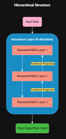
Figure 1: The multi-layered hierarchical organization of systemic neural resonance.
The Resonance Cycle (Adaptive Alignment Phase)
During explicit resonance prediction, ARCANE initializes states from the current input, constructs per-example top-down targets, and re-runs that same input for a configured number of cycles. Early stopping can occur when summed divergence falls below the configured threshold.
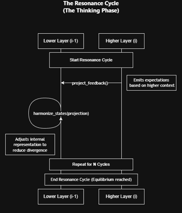
Figure 2: Information flow during hierarchical state synchronization.
Internal Logic of a ResonantGSER Layer
Each ResonantGSER layer exposes a per-example sequence summary and a feedback projection. The explicit loop passes batch-shaped targets directly; stored batch-mean variables exist only for legacy manual and callback compatibility.
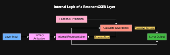
Figure 3: Local divergence calculation and state harmonization within the GSER cell.
Advantages and Disadvantages
Implemented properties
- Per-example targets: explicit inference does not collapse the batch into one prototype.
- Measurable alignment: adjacent-level reconstruction error and state divergence are exposed directly.
- Controlled compute: cycle count is configurable and can be compared from the same checkpoint.
- Reversible adaptation: optional fast-weight updates can be bounded, rolled back, and reset after each request.
Disadvantages and Limitations
Despite its theoretical advantages, the resonant approach introduces specific trade-offs:
- Compute and latency: every resonance cycle adds another forward evaluation of the current input.
- Objective mismatch: lower alignment divergence need not improve accuracy, calibration, or generation quality.
- Adaptation risk: entropy minimization and BCM can reinforce confident errors or introduce order sensitivity.
- Evidence limits: mechanism tests establish implementation behavior, not task superiority or biological equivalence.
Technical Implementation Details
The ARCANE framework implements this theory through two primary components:
1. The ResonantGSER Layer
The fundamental unit of the resonance hierarchy:
- Closed-form harmonization: EMA steps toward
resonance_alignment, skipped while that vector is unset. - Feedback Mechanism:
project_feedback()maps hidden→hidden by default;to_input_space=Trueusesfeedback_weights. - Per-example inference state:
predict_with_resonanceobtains(batch, units)sequence summaries and carries one target per example.last_his retained only as a batch-mean compatibility summary for legacy APIs. - Spikes: graded spikes, signed counts against a self-scaling threshold (
graded_spike), with a learned per-unit threshold and leak.
2. The NeuralResonanceCallback
Runs on on_train_batch_begin (before the current batch forward pass):
- Feedback Phase: Higher layers project from
last_h(previous batch prototype). - Harmonization Phase: Lower layers write that projection into
resonance_alignment. - Forward pass: The upcoming batch is attracted toward that prototype.
This callback is not an inner-loop re-forward of the current batch. Use predict_with_resonance for per-example hierarchical refinement, or PredictiveResonantLayer for local recurrent alignment.
Performance & Comparison
ARCANE includes exploratory comparisons and a controlled same-checkpoint ablation harness. The published example numbers below are historical smoke tests, not comprehensive validation.
Model Architectures Compared
| Architecture | Description | Key Features |
|---|---|---|
| Traditional Deep LSTM | 4-layer stacked LSTM | Pure feed-forward, no resonance |
| Neuromimetic (Standard) | NeuromimeticSemanticModel | 2-level ResonantGSER, Hebbian learning |
| Hierarchical Resonance | HierarchicalResonanceFoundationModel | Multi-level hierarchy, temporal coherence |
Tiny Shakespeare Benchmark (15,000 chars, 10 epochs)
These numbers are from a small exploratory run with unequal parameter counts. They are not a Transformer comparison and should only be treated as historical System 1 smoke-test results.
| Metric | Traditional LSTM | Neuromimetic (Standard) | Hierarchical Resonance |
|---|---|---|---|
| Validation Accuracy | 9.50% | 10.20% | 11.25% |
| Validation Loss | 6.85 | 6.42 | 6.15 |
| Training Time | ~45s | ~58s | ~95s |
| Parameters | ~195K | ~220K | ~385K |
| Reported loss variance | 0.0234 | 0.0189 | 0.0142 |
Training Dynamics Analysis
| Model | Convergence (90% final) | Loss Variance | Train/Val Gap |
|---|---|---|---|
| Traditional LSTM | Epoch 2 | 0.0234 | 0.082 |
| Neuromimetic (Standard) | Epoch 3 | 0.0189 | 0.065 |
| Hierarchical Resonance | Epoch 4 | 0.0142 | 0.048 |
MNIST (Spatio-Temporal Digit Classification)
| Metric | Traditional Deep LSTM | Resonant ARCANE |
|---|---|---|
| Test Accuracy | 98.76% | 98.89% |
| Test Loss | 0.0432 | 0.0391 |
| Training Time | ~947s | ~1518s |
Key Findings (exploratory, small data)
- Adding resonance levels changed Tiny Shakespeare accuracy by about one point at roughly 2× parameters.
- MNIST 98.89% vs 98.76% is within noise for that setup.
- Unit tests verify closed-form harmonization, STE spikes, and Keras 3 layer linking, not task superiority.
Implementation Example
from gpbacay_arcane import HierarchicalResonanceFoundationModelmodel = HierarchicalResonanceFoundationModel( vocab_size=5000, seq_len=32, hidden_dim=128, num_resonance_levels=4,)model.build_model()model.compile_model()model.model.fit(X_train, y_train)# Give feedback projections an explicit gradient path.model.train_feedback_step(X_train[:32], labels=y_train[:32])# Fixed-weight current-input refinement with per-example targets.predictions = model.predict_with_resonance(X_test, resonance_cycles=4)# Optional reversible weight adaptation.result = model.adapt_at_inference( X_test, variables="all", objective="entropy", steps=2, max_update_norm=1e-3, episodic=True,)Scientific Context
The mechanism is inspired by predictive-coding and recurrent-processing ideas. ARCANE implements engineering analogies such as top-down projections, local divergence, spiking transforms, and homeostatic traces, but does not establish neuroscientific fidelity.
Conclusion
Hierarchical Neural Resonance combines per-example state, differentiable feedback training, bounded test-time objectives, and a same-checkpoint ablation harness. Together, these features make recurrent refinement measurable and let each application select the cycle depth that best serves its accuracy and latency requirements.
Empirical Validation
The existing Tiny Shakespeare and MNIST numbers are exploratory, use limited seeds or unequal parameter counts, and do not isolate inference-time learning. A proper evaluation compares 0/1/2/4/8 cycles on the same checkpoint over multiple seeds and reports accuracy, negative log-likelihood, calibration, latency, forgetting, order sensitivity, batch-size sensitivity, and distribution shift.
Future Directions
- Evaluate whether alignment objectives correlate with downstream quality.
- Compare learned feedback with tied and identity feedback.
- Test persistent adaptation under ordering and distribution shifts.
- Profile cycle latency and memory at realistic sequence lengths.